The Economist magazine just published an article that talked about "synthetic" hedge funds, or replicating hedge fund returns using factor models. The original research cited can be found here. (For those of you who want a primer on factor models, I have written an article on this topic previously.) The seven factors are (are you ready?):
1) excess return on the S&P 500 index;
2) a small minus big factor constructed as the difference of the Wilshire small and large
capitalization stock indices;
3) excess returns on portfolios of lookback straddle options on currencies;
4) excess returns on portfolios of lookback straddle options on commodities;
5) excess returns on portfolios of lookback straddle options on bonds;
6) the yield spread of the US ten year treasury bond over the three month T-bill, adjusted for the duration of the ten year bond;
7) the change in the credit spread of the Moody's BAA bond over the 10 year treasury bond, also appropriately adjusted for duration.
According to the researchers, factors 3)-5) are constructed to replicate the maximum possible return to trend-following strategies on their respective underlying assets.
See, it is not that difficult to run a hedge fund after all!
Saturday, March 24, 2007


Sunday, March 18, 2007
Is increasing beta or increasing leverage a better way to increase returns?
In my previous post, I reported an astute observation from my reader Mr. Goldstein that maximizing compound rate of return, maximizing leverage, and maximizing Sharpe ratio are all tightly connected. This makes intuitive sense because the higher the Sharpe ratio of a strategy, the smaller the drawdown, and therefore the higher the leverage you can apply to it in order to maximize compound return.
Mr. Goldstein also made another very interesting observation. He noted that there are usually 2 ways to increase the returns of a portfolio of stocks: either by picking high-beta stocks, or by increasing the leverage of the portfolio. In both cases, we are taking on more risk in order to generate more returns. But are these 2 ways equal? Or is one better than the other? It turns out that there is some research out there which suggests increasing leverage is the better way, due to the fact that the market seems to be chronically under-pricing high-beta stocks. This gives rise to a strategy called "Beta Arbitrage": buy low-beta stocks, short high-beta stocks, and earn a positive return.
I myself have not studied this form of arbitrage in depth, and therefore can neither endorse nor criticize it. However, if this research is correct, it does argue against including too many volatile stocks in your portfolio or trading strategy. If you want to take on more risk and generate higher return, just turn the knob and increase your leverage and therefore book size.
Mr. Goldstein also made another very interesting observation. He noted that there are usually 2 ways to increase the returns of a portfolio of stocks: either by picking high-beta stocks, or by increasing the leverage of the portfolio. In both cases, we are taking on more risk in order to generate more returns. But are these 2 ways equal? Or is one better than the other? It turns out that there is some research out there which suggests increasing leverage is the better way, due to the fact that the market seems to be chronically under-pricing high-beta stocks. This gives rise to a strategy called "Beta Arbitrage": buy low-beta stocks, short high-beta stocks, and earn a positive return.
I myself have not studied this form of arbitrage in depth, and therefore can neither endorse nor criticize it. However, if this research is correct, it does argue against including too many volatile stocks in your portfolio or trading strategy. If you want to take on more risk and generate higher return, just turn the knob and increase your leverage and therefore book size.
Sunday, March 04, 2007
Maximizing Compound Rate of Return vs Maximizing Sharpe ratio
A reader, Mr. A. Goldstein, made a very useful observation about my article "Maximizing Compound Rate of Return". In that article I argued that if your goal is to maximize the compound rate of return, you should maximize the quantity m – s2/2, where m is the short-term (1-period) rate of return, and s is its standard deviation. In general, this is not the same as maximizing the Sharpe ratio of a strategy. However, Mr. Goldstein pointed out that, if you also optimize the leverage of your strategy using Kelly's criterion, then maximizing Sharpe ratio does in fact maximize the compound rate of return also. This follows from a calculation in section 7 of Dr. Edward Thorpe's paper www.bjmath.com/bjmath/thorp/paper.htm.
Mr. Goldstein also suggested a beta arbitrage strategy which he has allowed me to share with my readers in a future post.
Mr. Goldstein also suggested a beta arbitrage strategy which he has allowed me to share with my readers in a future post.
Tuesday, February 27, 2007
Platinum-gold spread revisited
Now that Chinese New Year is over, it is time to revisit the Platinum-Gold spread that I talked about last November. The theory is that with the demand for gold seasonally exhausted due to the end of Asian festivities, gold prices will decline relative to platinum. We now have the opportunity to test this theory again.
Saturday, February 24, 2007
Index arbitrage with XLE
In looking for pairs of financial instruments to pair trade, we do not have to limit ourselves to pairs that occur in "nature". We can often construct our own baskets of stocks to trade against an index (or an ETF representing this index). In fact, such pairs usually show better cointegration properties than any stock or ETF pairs. I have alluded to this index arbitrage idea in an earlier post, and the details of the methodology are explained in my articles for Subscribers. I tried this strategy on favorite sector ETF: the energy SPDR XLE.
XLE is composed of some 33 stocks (as of 2/16/2007). Our goal is to pick some smaller subset of these stocks to form a basket. We pick them based on how well they cointegrate with XLE. How big should this subset be? The higher the number, the better this basket cointegrates with XLE, but the smaller the profits. (If you include all stocks in XLE in this basket, then the basket cointegrates perfectly with XLE, but there will be no trading opportunities!) The lower the number, the higher the (specific) risk as well as return. So it is more of a personal risk-return preference than any scientific criterion which determines how many stocks to pick. I pick a basket with 10 stocks. I have found that this basket cointegrates with XLE with better than 99% probability since 2001/05/22. The half-life for mean-reversion is about 20 days, which means you have to hold a position for at most a quarter. (My own rule is to exit when the spread hasn't reverted in 3 times the half-life.) If you enter into a position when the z-score is about ±2, you can expect a profit of about $2,000 on an investment of about $58,000 on one side. This comes to a return per trade of about 3%. You can of course boost this return by using options to implement the XLE position instead.
As an aside, if you use Interactive Brokers, you can easily trade an entire basket of stocks using their Basket Trader.
I have created an online spreadsheet with (almost) real-time values of this spread in the subscription area. (The detailed composition of this basket of 10 stocks are also described there.) Note that in theory, every time the XLE changes composition, we will have to re-compute our basket composition as well. But fortunately XLE composition does not change very much or very often, so I will only update my basket at most once a month.
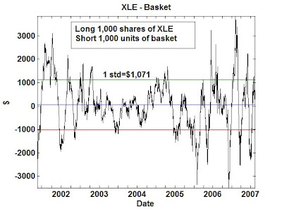
XLE is composed of some 33 stocks (as of 2/16/2007). Our goal is to pick some smaller subset of these stocks to form a basket. We pick them based on how well they cointegrate with XLE. How big should this subset be? The higher the number, the better this basket cointegrates with XLE, but the smaller the profits. (If you include all stocks in XLE in this basket, then the basket cointegrates perfectly with XLE, but there will be no trading opportunities!) The lower the number, the higher the (specific) risk as well as return. So it is more of a personal risk-return preference than any scientific criterion which determines how many stocks to pick. I pick a basket with 10 stocks. I have found that this basket cointegrates with XLE with better than 99% probability since 2001/05/22. The half-life for mean-reversion is about 20 days, which means you have to hold a position for at most a quarter. (My own rule is to exit when the spread hasn't reverted in 3 times the half-life.) If you enter into a position when the z-score is about ±2, you can expect a profit of about $2,000 on an investment of about $58,000 on one side. This comes to a return per trade of about 3%. You can of course boost this return by using options to implement the XLE position instead.
As an aside, if you use Interactive Brokers, you can easily trade an entire basket of stocks using their Basket Trader.
I have created an online spreadsheet with (almost) real-time values of this spread in the subscription area. (The detailed composition of this basket of 10 stocks are also described there.) Note that in theory, every time the XLE changes composition, we will have to re-compute our basket composition as well. But fortunately XLE composition does not change very much or very often, so I will only update my basket at most once a month.

Thursday, February 15, 2007
Do Gold and Oil Cointegrate?
I have written extensively here about cointegration between gold-miners and gold ETF's (GDX vs GLD), as well as between energy companies and oil ETF's (XLE vs USO). (See, for e.g., this article, or this article.) On another occasion, I also commented on an Economist magazine article about the possible cointegration between bond yield and oil prices. However, my fellow blogger Yaser recently pointed out an interesting link between gold and oil also. The reasons why gold and oil may be cointegrated are very similar to that of bond yield and oil: as oil price rise a) the oil revenue is invested heavily in gold, therefore pushing up gold price; b) there is an upward pressure on inflation, which increases the appeal of gold as an inflation hedge.
I did a cointegration analysis between gold and oil prices, and though their spread certainly looks somewhat mean-reverting since the 90's, it doesn't pass the cointegration test. The reason may simply be that this spread mean-reverts at a glacial pace: I estimate that the half-life (see my explanation of this term here) is over 14 months. Therefore, it may require historical data back to the 1970's to convince ourselves of their cointegration. (My own data on crude oil and gold prices only go as far back as the 1990's. If any reader knows of historical data source that goes back further, please let me know.) If, however, one is willing to take their cointegration by faith despite the inadequate data, then one may believe that gold is currently (as of Feb 12, 2007) just slightly undervalued relative to oil (the spread is about $8). I certainly don't recommend entering into a position on either side at this point!

I did a cointegration analysis between gold and oil prices, and though their spread certainly looks somewhat mean-reverting since the 90's, it doesn't pass the cointegration test. The reason may simply be that this spread mean-reverts at a glacial pace: I estimate that the half-life (see my explanation of this term here) is over 14 months. Therefore, it may require historical data back to the 1970's to convince ourselves of their cointegration. (My own data on crude oil and gold prices only go as far back as the 1990's. If any reader knows of historical data source that goes back further, please let me know.) If, however, one is willing to take their cointegration by faith despite the inadequate data, then one may believe that gold is currently (as of Feb 12, 2007) just slightly undervalued relative to oil (the spread is about $8). I certainly don't recommend entering into a position on either side at this point!


Wednesday, February 14, 2007
Another article on political futures markets
A NYTimes article yesterday talked about the political futures market intrade.com in the context of the November election, particularly the Virginia Senate race, which I blogged about before. I urged my readers to curb their enthusiasm for using such markets for prediction in my article, while the NYTimes article is certainly much more enamored of them. However, I think we can all agree that such markets are very efficient in synthesizing all existing information and opinion in making a prediction, but it cannot reveal information that nobody can possibly know at this point, such as who is going to win the 2008 general election.
Monday, February 12, 2007
Use the right discount rate to avoid jail time
Here is a fascinating story about the former treasurer of Essex County, New Jersey, who was sentenced to seven and a half years in prison because the prosecutor used the wrong discount rate to value certain tax-exempt bonds.
Saturday, February 10, 2007
In praise of day-trading
A recent article by Mark Hulbert in the NYTimes talked about the Value Line's rankings, and how this system is under-performing the market index in recent years. Mr. Hulbert asked Professor David Aronson of Baruch College whether this drop in performance means that the system has stopped working. Prof. Aronson says no: he believes that it takes 10 or more years [my emphasis] of under-performance of this strategy before one can say that it has stopped working! This statement, if taken out-of-context, is so manifestly untrue that it warrants some elaboration.
To evaluate whether a strategy has failed bears a lot of resemblance to evaluating whether a particular trade has failed. In my previous article on stop-loss, I outlined a method to determine how long it takes before we should exit a losing trade. This has to do with the historical average holding period of similar trades. This kind of thinking can also be applied to a strategy as a whole. If your strategy, like the Value Line system, holds a position for months or even years before replacing it with others, then yes, it may take many years to find out if the system has finally stopped working. On the other hand, if your system holds a position for just hours, or maybe just minutes, then no, it takes only a few months to find out! Why? Those who are well-versed in statistics know that the larger the sample size (in this case, the number of trades), the smaller the percent deviation from the mean return.
Which brings me to day-trading. In the popular press, day-trading has been given a bad-name. Everyone seems to think that those people who sit in sordid offices buying and selling stocks every minute and never holding over-night positions are no better than gamblers. And we all know how gamblers end up, right? Let me tell you a little secret: in my years working for hedge funds and prop-trading groups in investment banks, I have seen all kinds of trading strategies. In 100% of the cases, traders who have achieved spectacularly high Sharpe ratio (like 6 or higher), with minimal drawdown, are day-traders.
To evaluate whether a strategy has failed bears a lot of resemblance to evaluating whether a particular trade has failed. In my previous article on stop-loss, I outlined a method to determine how long it takes before we should exit a losing trade. This has to do with the historical average holding period of similar trades. This kind of thinking can also be applied to a strategy as a whole. If your strategy, like the Value Line system, holds a position for months or even years before replacing it with others, then yes, it may take many years to find out if the system has finally stopped working. On the other hand, if your system holds a position for just hours, or maybe just minutes, then no, it takes only a few months to find out! Why? Those who are well-versed in statistics know that the larger the sample size (in this case, the number of trades), the smaller the percent deviation from the mean return.
Which brings me to day-trading. In the popular press, day-trading has been given a bad-name. Everyone seems to think that those people who sit in sordid offices buying and selling stocks every minute and never holding over-night positions are no better than gamblers. And we all know how gamblers end up, right? Let me tell you a little secret: in my years working for hedge funds and prop-trading groups in investment banks, I have seen all kinds of trading strategies. In 100% of the cases, traders who have achieved spectacularly high Sharpe ratio (like 6 or higher), with minimal drawdown, are day-traders.
Monday, February 05, 2007
Index tracking, arbitrage, and cointegration
Mr. Lange, a reader of mine from Germany, alerted me to the following paper regarding a strategy related to index arbitrage that involves the EUROStoxx50 index. It is a nice illustration of a common application of cointegration techniques to statistical arbitrage trading. I have written an exposition of this paper, together with an additional index arbitrage strategy not discussed in the original paper, which I posted to my subscribers only area. (Mr. Lange has graciously allowed me to share this exposition with other readers of this blog.)
Sunday, February 04, 2007
Cointegration between oil and bond yield? Not!
An article in the Feb 1 issue of the Economist magazine suggested that there may be a link between crude oil price and long-dated US treasuries. Their reasoning is that if oil price is high, OPEC will need to re-invest the pile of cash that they generate, and eventually a lot of this ended up invested in US 10-year bond. Therefore, when crude prices go up, 10-year yield should go down. As I explained before, the fact that these 2 numbers are anti-correlated do not prevent them from being cointegrated. And in fact, the Economist article plotted the crude oil prices together with bond yield over the last year together, and they seem tantalizingly close to being cointegrated.
My curiosity piqued, I proceeded to get a longer history of these data to examine.
 In the graph above, I plotted the (normalized) difference between the 10-year treasury yield and oil price. One can see that over the last year and a half, they are indeed cointegrated to a good degree. (To see that, notice the spread is range-bound, or mean-reverting, from mid-2005 to the present.) But this relationship breaks down completely over the longer history.
Though I think that the Economist magazine is doing a disservice to its readers for plotting this graph over just one year and making innuendos of linkage, it is a nice illustration of the danger of studying cointegration over a short window.
My curiosity piqued, I proceeded to get a longer history of these data to examine.
 In the graph above, I plotted the (normalized) difference between the 10-year treasury yield and oil price. One can see that over the last year and a half, they are indeed cointegrated to a good degree. (To see that, notice the spread is range-bound, or mean-reverting, from mid-2005 to the present.) But this relationship breaks down completely over the longer history.
Though I think that the Economist magazine is doing a disservice to its readers for plotting this graph over just one year and making innuendos of linkage, it is a nice illustration of the danger of studying cointegration over a short window.
Sunday, January 28, 2007
Stop-loss strategy: re-post
Due to a technical glitch, many subscribers to this blog were not notified of my latest article on stop-loss strategy and a method to estimate optimal holding period for mean-reverting strategies.
So here is the permanent link again.
So here is the permanent link again.
Monday, January 15, 2007
What is your stop loss strategy?
A reader recently asked me whether setting a stop loss for a trading strategy is a good idea. I am a big fan of setting stop loss, but there are certainly myriad views on this.
One of my former bosses didn't believe in stop loss: his argument is that the market does not care about your personal entry price, so your stop price may be somebody else’s entry point. So stop loss, to him, is irrational. Since he is running a portfolio with hundreds of positions, he doesn’t regard preserving capital in just one or a few specific positions to be important. Of course, if you are an individual trader with fewer than a hundred positions, preservation of capital becomes a lot more important, and so does stop loss.
Even if you are highly diversified and preservation of capital in specific positions is not important, are there situations where stop loss is rational? I certainly think that applies to trend-following strategies. Whenever you incur a big loss when you have a trend-following position, it ususally means that the latest entry signal is opposite to your original entry signal. In this case, better admit your mistake, close your position, and maybe even enter into the opposite side. (Sometimes I wish our politicians think this way.) On the other hand, if you employ a mean-reverting strategy, and instead of reverting, the market sticks to its original direction and causes you to lose money, does it mean you are wrong? Not necessarily: you could simply be too early. Indeed, many traders in this case will double up their position, since the latest entry signal in this case is in the same direction as the original one. This raises a question though: if incurring a big loss is not a good enough reason to surrender to the market, how would you ever decide if your mean-reverting model is wrong? Here I propose a stop loss criterion that looks at another dimension: time.
The simplest model one can apply to a mean-reverting process is the Ornstein-Uhlenbeck formula. As a concrete example, I will apply this model to the commodity ETF spreads I discussed before that I believe are mean-reverting (XLE-CL, GDX-GLD, EEM-IGE, and EWC-IGE). It is a simple model that says the next change in the spread is opposite in sign to the deviation of the spread from its long-term mean, with a magnitude that is proportional to the deviation. In our case, this proportionality constant θ can be estimated from a linear regression of the daily change of the spread versus the spread itself. Most importantly for us, if we solve this equation, we will find that the deviation from the mean exhibits an exponential decay towards zero, with the half-life of the decay equals ln(2)/θ. This half-life is an important number: it gives us an estimate of how long we should expect the spread to remain far from zero. If we enter into a mean-reverting position, and 3 or 4 half-life’s later the spread still has not reverted to zero, we have reason to believe that maybe the regime has changed, and our mean-reverting model may not be valid anymore (or at least, the spread may have acquired a new long-term mean.)
Let’s now apply this formula to our spreads and see what their half-life’s are. Fitting the daily change in spreads to the spread itself gives us:
These numbers do confirm my experience that the GDX-GLD spread is the best one for traders, as it reverts the fastest, while the XLE-CL spread is the most trying. If we arbitrarily decide that we will exit a spread once we have held it for 3 times the half-life, we have to hold the XLE-CL spread almost a calendar year before giving up. (Note that the half-life count only trading days.) And indeed, while I have entered and exited (profitably) the GDX-GLD spread several times since last summer, I am holding the XLE - QM (substituting QM for CL) spread for the 104th day!
Sentiment as contrarian indicator
More insights from Steve on using sentiment as contrarian indicator. (See his comments on my article on Market-cap and growth-value arbitrage.)
Sunday, January 14, 2007
Factor models: the debate continues...
A reader JR just posted some very thoughtful comments on my article on factor models. You can read his comments and my reply here.
Thursday, January 11, 2007
Quantitative sports betting
Here is an interesting WSJ article on a statistician who makes an excellent living betting on sports, quantitatively. (Thanks to my friend Steve Halpern for the tip!)
Sunday, January 07, 2007
Universal Portfolios
Let me describe a portfolio optimization scheme that, over the long run, is supposedly guaranteed to outperform the best stock in the portfolio.
Before we begin, let’s agree that we will rebalance our portfolio every day so that each stock has a fixed percent allocation of capital, just as your favorite financial consultant would have advised you. What this means is that if you own IBM and MSFT, and IBM went up after one day whereas MSFT went down, you should sell some IBM and use the capital to buy some more MSFT. There is a technical term for such portfolios: they are called “constant rebalanced portfolios”. Notice also the similarity with the Kelly criterion which I wrote about before: Kelly criterion asks you to maintain a constant leverage, which is like maintaining a fixed percent allocation between cash (debt) and stock.
But what should the fixed percent allocation be? Here is where the scheme gets interesting. Suppose we start with an equal capital allocation, for lack of any better choice. At the end of the day, your portfolio has a certain net worth. But then you can calculate what the net worth would have turned out if you had started with a different allocation. Indeed, we can run this simulation: try all possible initial allocations, and calculate the hypothetical net worth of the resulting portfolio. Use these hypothetical net worth as weights (after normalizing them by the sum of all net worth), and compute a weighted-average percent allocation. Finally, adopt this weighted average allocation as the new desired allocation and rebalance the portfolio accordingly. So actually the “fixed” percent allocation is not fixed after-all: it gets adjusted daily, but probably not by much. Repeat this process everyday, always calculating a new weighted allocation by simulating various initial allocations since day 1.
This scheme of portfolio optimization can be proven to produce a net worth greater than just holding the best stock, given long enough time. If this sounds like a miracle, it is partly because this is in fact an ingenious result of information theory, and partly because there are various caveats that actually limit its practical application. The proof that it works (at least in theory) is rather technical and I will let the interested reader peruse the original paper published by Prof. Thomas Cover, a noted information theorist from Stanford University. He coined the term “Universal Portfolios” for portfolios rebalanced/optimized with this scheme. Without understanding the mathematical intuition, this scheme may appeal to those who believe in long-term trending behavior of stocks, because if a stock performs very well in the past, we will end up allocating more capital to it in the long run. It may also appeal to those who believe in short-term mean reversal behavior, since in the short-term, we are performing daily rebalancing of the stock positions based on an approximately constant allocation. However, this seeming confirmation of either trending or mean-reverting characteristics of stock prices is illusory – this scheme is supposed to work even if the stock prices are totally random! How can we manage to squeeze out a gain even with random price series? Remember that we have done the opposite before (see my earlier articles): we manage to lose money even when a price series exhibits a geometric random walk. So it is not too surprising that we can also make money using similar information theoretic juggling.
Now for the caveats. Every time an information theorist start saying “In the long run, …”, you will be well-advised to ask: How long? In my geometric random walk example where the volatility (standard deviation) of returns every period is 1%, we find that the compounded rate of return is an agonizingly small -0.005% per period. In the case of the universal portfolio scheme, the out-performance over the best stock in the portfolio is similarly dependent on the volatilities of the stocks: the higher the volatility, the faster the out-performance. Let me run a simulation with a portfolio consisting of two ETF’s RTH and OIH. If we were to run the Universal Portfolio scheme from 2001/5/17 – 2006/12/29, I find that the cumulative return is 32% (without transaction cost). Contrast that with just buying-and-holding the best ETF (namely OIH here): the cumulative return is 54%. The Universal Portfolio loses. Does this mean the theory is wrong? Not really: RTH and OIH may just have too low volatility. Herein lies the first practical caveat with the Universal Portfolio scheme: it can take too long to realize its benefit if the volatility is low.
How do we find ETF’s that have high enough volatility to realize the out-performance of Universal Portfolio? Actually, we can simply boost the volatility of RTH and OIH artificially by increasing their leverage. So let’s say we leverage both of them 2x. This means their daily returns and volatilities are both doubled. Now the best ETF (which is still OIH here) has a return of 23% (why is it lower than the un-leveraged case? Remember the formula m-s2/2 in my previous article.) , but the Universal Portfolio has a return of 45%. So now the Universal Portfolio wins. But this is a Pyrrhic victory: if you factor in a transaction cost of 10 basis points, the Universal Portfolio scheme actually returns only 4%. This is the second caveat of Universal Portfolios: because of the frequent rebalancing required, transaction costs tend to eat up all the out-performance.
Now there is a final caveat. The reader may ask why I don’t just pick two stocks instead of two ETF’s to illustrate this scheme. Aren’t most stocks more volatile than ETF’s and therefore much better suited for this scheme? Indeed, most academic papers, including Prof. Cover’s original paper, use a pair of stocks for illustration. But if we do that, we run the risk of introducing survivorship bias. Naturally, if you know ahead of time that none of these two stocks will go bankrupt, the Universal Portfolio scheme may look great. But if you run a simulation where one of the stocks suddenly went bankrupt one day (which tend to be a fairly mathematically discontinuous affair), the Universal Portfolio scheme will most likely not beat holding just the non-bankrupt stock in the beginning. Using ETF’s eliminated this problem. But then ETF’s are far less volatile.
So given all these caveats, is Universal Portfolio really practical? Prof. Cover seems to think so. That’s why he has started a hedge fund to prove it.
Before we begin, let’s agree that we will rebalance our portfolio every day so that each stock has a fixed percent allocation of capital, just as your favorite financial consultant would have advised you. What this means is that if you own IBM and MSFT, and IBM went up after one day whereas MSFT went down, you should sell some IBM and use the capital to buy some more MSFT. There is a technical term for such portfolios: they are called “constant rebalanced portfolios”. Notice also the similarity with the Kelly criterion which I wrote about before: Kelly criterion asks you to maintain a constant leverage, which is like maintaining a fixed percent allocation between cash (debt) and stock.
But what should the fixed percent allocation be? Here is where the scheme gets interesting. Suppose we start with an equal capital allocation, for lack of any better choice. At the end of the day, your portfolio has a certain net worth. But then you can calculate what the net worth would have turned out if you had started with a different allocation. Indeed, we can run this simulation: try all possible initial allocations, and calculate the hypothetical net worth of the resulting portfolio. Use these hypothetical net worth as weights (after normalizing them by the sum of all net worth), and compute a weighted-average percent allocation. Finally, adopt this weighted average allocation as the new desired allocation and rebalance the portfolio accordingly. So actually the “fixed” percent allocation is not fixed after-all: it gets adjusted daily, but probably not by much. Repeat this process everyday, always calculating a new weighted allocation by simulating various initial allocations since day 1.
This scheme of portfolio optimization can be proven to produce a net worth greater than just holding the best stock, given long enough time. If this sounds like a miracle, it is partly because this is in fact an ingenious result of information theory, and partly because there are various caveats that actually limit its practical application. The proof that it works (at least in theory) is rather technical and I will let the interested reader peruse the original paper published by Prof. Thomas Cover, a noted information theorist from Stanford University. He coined the term “Universal Portfolios” for portfolios rebalanced/optimized with this scheme. Without understanding the mathematical intuition, this scheme may appeal to those who believe in long-term trending behavior of stocks, because if a stock performs very well in the past, we will end up allocating more capital to it in the long run. It may also appeal to those who believe in short-term mean reversal behavior, since in the short-term, we are performing daily rebalancing of the stock positions based on an approximately constant allocation. However, this seeming confirmation of either trending or mean-reverting characteristics of stock prices is illusory – this scheme is supposed to work even if the stock prices are totally random! How can we manage to squeeze out a gain even with random price series? Remember that we have done the opposite before (see my earlier articles): we manage to lose money even when a price series exhibits a geometric random walk. So it is not too surprising that we can also make money using similar information theoretic juggling.
Now for the caveats. Every time an information theorist start saying “In the long run, …”, you will be well-advised to ask: How long? In my geometric random walk example where the volatility (standard deviation) of returns every period is 1%, we find that the compounded rate of return is an agonizingly small -0.005% per period. In the case of the universal portfolio scheme, the out-performance over the best stock in the portfolio is similarly dependent on the volatilities of the stocks: the higher the volatility, the faster the out-performance. Let me run a simulation with a portfolio consisting of two ETF’s RTH and OIH. If we were to run the Universal Portfolio scheme from 2001/5/17 – 2006/12/29, I find that the cumulative return is 32% (without transaction cost). Contrast that with just buying-and-holding the best ETF (namely OIH here): the cumulative return is 54%. The Universal Portfolio loses. Does this mean the theory is wrong? Not really: RTH and OIH may just have too low volatility. Herein lies the first practical caveat with the Universal Portfolio scheme: it can take too long to realize its benefit if the volatility is low.
How do we find ETF’s that have high enough volatility to realize the out-performance of Universal Portfolio? Actually, we can simply boost the volatility of RTH and OIH artificially by increasing their leverage. So let’s say we leverage both of them 2x. This means their daily returns and volatilities are both doubled. Now the best ETF (which is still OIH here) has a return of 23% (why is it lower than the un-leveraged case? Remember the formula m-s2/2 in my previous article.) , but the Universal Portfolio has a return of 45%. So now the Universal Portfolio wins. But this is a Pyrrhic victory: if you factor in a transaction cost of 10 basis points, the Universal Portfolio scheme actually returns only 4%. This is the second caveat of Universal Portfolios: because of the frequent rebalancing required, transaction costs tend to eat up all the out-performance.
Now there is a final caveat. The reader may ask why I don’t just pick two stocks instead of two ETF’s to illustrate this scheme. Aren’t most stocks more volatile than ETF’s and therefore much better suited for this scheme? Indeed, most academic papers, including Prof. Cover’s original paper, use a pair of stocks for illustration. But if we do that, we run the risk of introducing survivorship bias. Naturally, if you know ahead of time that none of these two stocks will go bankrupt, the Universal Portfolio scheme may look great. But if you run a simulation where one of the stocks suddenly went bankrupt one day (which tend to be a fairly mathematically discontinuous affair), the Universal Portfolio scheme will most likely not beat holding just the non-bankrupt stock in the beginning. Using ETF’s eliminated this problem. But then ETF’s are far less volatile.
So given all these caveats, is Universal Portfolio really practical? Prof. Cover seems to think so. That’s why he has started a hedge fund to prove it.
Tuesday, December 26, 2006
Do Factor Models Work in the Short Term?
Besides pair-trading, “factor model” is the most popular workhorse of the statistical arbitrageur. In a previous article, I discussed the most well-known factor model – the Fama-French Three-Factor model, with the general market index returns, the market-cap of the stock, and the book-to-price ratio as the only three factors driving returns. However, as I explained earlier, this factor model has a very long horizon. For the quantitative trader who needs to make money every month, the natural instinct is to look for a more “sophisticated” factor that works in the short term, or even to develop some kind of model that use different factors every month in response to “market condition”. Alas, other than hearsays and second-hand gossips, I have never witnessed an actual success of this approach in a hedge fund or proprietary trading group – at least a success that lasts for more than a year.
I am of course not privy to the current performance numbers of factor models run by some of the most successful hedge funds today. However, there is a class of ETF (called “XTF”) marketed by PowerShares Capital Management that uses a similar factor approach for its stock selection criteria. According to media reports, each stock in these XTF’s is scored by 25 variables such as cash flow, earnings growth, price momentum, etc. This sounds like a classic factor model to me. This model is reportedly designed by the quantitative unit at American Stock Exchange. To find out if they have indeed discovered the holy grail of factor models, I looked at the performance of these XTF compared to their benchmarks.
Here I tabulate the XTF’s for each market cap and value category, their corresponding benchmark market index ETF’s, and finally the YTD differential returns up to December 13, 2006. (PJG and PJM have too short a history for this comparison.)
The differential returns are all over the place: some positive, others negative. To me, this is symptomatic of a factor model that does not have predictive power. (After all, if the differential returns are consistently negative, we could have long the ETF, short the XTF, and make consistent profits!) At the very least, this factor model may have a horizon much longer than what most traders would be interested in – in which case, why not just use the simple Fama-French model?
This is not to say that exotic, proprietary factor models have no use: they tend to be pretty useful for risk management, as volatilities and correlations are often easier to predict than returns. But beware every time your risk management software vendor tries to sell you an alpha generator!
I am of course not privy to the current performance numbers of factor models run by some of the most successful hedge funds today. However, there is a class of ETF (called “XTF”) marketed by PowerShares Capital Management that uses a similar factor approach for its stock selection criteria. According to media reports, each stock in these XTF’s is scored by 25 variables such as cash flow, earnings growth, price momentum, etc. This sounds like a classic factor model to me. This model is reportedly designed by the quantitative unit at American Stock Exchange. To find out if they have indeed discovered the holy grail of factor models, I looked at the performance of these XTF compared to their benchmarks.
Here I tabulate the XTF’s for each market cap and value category, their corresponding benchmark market index ETF’s, and finally the YTD differential returns up to December 13, 2006. (PJG and PJM have too short a history for this comparison.)
| Value | Blend | Growth | |
| Large cap | PWV-IVE=4.8% | PWC-IVV=-3.6% | PWB-IVW=-5.0% |
| Mid cap | PWP-IJJ=0.1% | PJG-IJH=N/A | PWJ-IJK=3.1% |
| Small cap | PWY-IJS=-0.7% | PJM-IJR=N/A | PWT-IJT=-4.9% |
The differential returns are all over the place: some positive, others negative. To me, this is symptomatic of a factor model that does not have predictive power. (After all, if the differential returns are consistently negative, we could have long the ETF, short the XTF, and make consistent profits!) At the very least, this factor model may have a horizon much longer than what most traders would be interested in – in which case, why not just use the simple Fama-French model?
This is not to say that exotic, proprietary factor models have no use: they tend to be pretty useful for risk management, as volatilities and correlations are often easier to predict than returns. But beware every time your risk management software vendor tries to sell you an alpha generator!
Tuesday, December 19, 2006
Another limitation of artificial intelligence and data mining
Sometime ago I espoused my views that AI and data mining techniques may not be suited for predicting financial markets. Here we have an article from the Chief Scientist at IBM's Entity Analytic Solutions Group who believes these techniques are not fit for counterterrorism either. Why? The same reasons I mentioned: not enough historical data.
Thursday, December 14, 2006
DNA, cryptology, speech recognition, and trading
There is an interesting New York Times article on a mathematician and cryptologist who used to work for the wildly successful hedge fund Renaissance Technologies and is now famous for decoding DNA's. This article caught my eyes because quite a few of my former colleagues from the speech recognition research group at IBM also went over to Renaissance as researchers and portfolio managers. Renaissance is an extraordinary hedge fund in Long Island that has an average annual return of 35% since 1989, after charging 5% management fee and 44% incentive fee. They profess to hire only scientists, engineers and mathematicians with as little background in finance as possible. They started off trading futures, but has since then diversified into equities models, and is reportedly raising a $100 billion fund at the moment.
A lot of people want to know the secrets of their success. From the people they hire, one can always guess. The common thread among DNA decoding, cryptography, and speech recognition is information theory, the discipline founded by legendary Bell Labs mathematician Claude Shannon. There are a few tools in information theory that have found wide-spread applications: hidden Markov model is one, expectation-maximization (EM) algorithm is another, and then of course the grandfather of prediction: Bayesian statistics. Needless to say, I have tried them all in my own trading research, but have not met much success so far. Aside from the limitations of my imagination, I suspect the reason is that these tools work much better with higher frequency data than the daily data that I have thus far worked with. Therefore I am not ready to give up yet. (Readers of my earlier article on artificial intelligence may think that I am being inconsistent here, as I was less than enthusiastic about the application of that discipline to trading. There is, however, quite a big difference between information theory and artificial intelligence. The former is characterized by sophisticated theory with very few parameters, the latter, simple theory with a lot of parameters.)
There is one published trading model that is based squarely on research in information theory. It is called Universal Portfolios, created by Stanford information theorist Prof. Thomas Cover. It is an elegant and quite intuitive model, but I don't know how well it performs under realistic conditions. I hope to write about some of my research on this and a related class of models in a future article.
Further reading:
Cover, Thomas M. and Thomas, Joy A. (1991), Elements of Information Theory. John Wiley & Sons, Inc.
A lot of people want to know the secrets of their success. From the people they hire, one can always guess. The common thread among DNA decoding, cryptography, and speech recognition is information theory, the discipline founded by legendary Bell Labs mathematician Claude Shannon. There are a few tools in information theory that have found wide-spread applications: hidden Markov model is one, expectation-maximization (EM) algorithm is another, and then of course the grandfather of prediction: Bayesian statistics. Needless to say, I have tried them all in my own trading research, but have not met much success so far. Aside from the limitations of my imagination, I suspect the reason is that these tools work much better with higher frequency data than the daily data that I have thus far worked with. Therefore I am not ready to give up yet. (Readers of my earlier article on artificial intelligence may think that I am being inconsistent here, as I was less than enthusiastic about the application of that discipline to trading. There is, however, quite a big difference between information theory and artificial intelligence. The former is characterized by sophisticated theory with very few parameters, the latter, simple theory with a lot of parameters.)
There is one published trading model that is based squarely on research in information theory. It is called Universal Portfolios, created by Stanford information theorist Prof. Thomas Cover. It is an elegant and quite intuitive model, but I don't know how well it performs under realistic conditions. I hope to write about some of my research on this and a related class of models in a future article.
Further reading:
Cover, Thomas M. and Thomas, Joy A. (1991), Elements of Information Theory. John Wiley & Sons, Inc.
Subscribe to:
Posts (Atom)