Stop-loss strategy: re-post

Due to a technical glitch, many subscribers to this blog were not notified of my latest article on stop-loss strategy and a method to estimate optimal holding period for mean-reverting strategies.
So here is the permanent link again.

What is your stop loss strategy?

A reader recently asked me whether setting a stop loss for a trading strategy is a good idea. I am a big fan of setting stop loss, but there are certainly myriad views on this.

One of my former bosses didn't believe in stop loss: his argument is that the market does not care about your personal entry price, so your stop price may be somebody else’s entry point. So stop loss, to him, is irrational. Since he is running a portfolio with hundreds of positions, he doesn’t regard preserving capital in just one or a few specific positions to be important. Of course, if you are an individual trader with fewer than a hundred positions, preservation of capital becomes a lot more important, and so does stop loss.

Even if you are highly diversified and preservation of capital in specific positions is not important, are there situations where stop loss is rational? I certainly think that applies to trend-following strategies. Whenever you incur a big loss when you have a trend-following position, it ususally means that the latest entry signal is opposite to your original entry signal. In this case, better admit your mistake, close your position, and maybe even enter into the opposite side. (Sometimes I wish our politicians think this way.) On the other hand, if you employ a mean-reverting strategy, and instead of reverting, the market sticks to its original direction and causes you to lose money, does it mean you are wrong? Not necessarily: you could simply be too early. Indeed, many traders in this case will double up their position, since the latest entry signal in this case is in the same direction as the original one. This raises a question though: if incurring a big loss is not a good enough reason to surrender to the market, how would you ever decide if your mean-reverting model is wrong? Here I propose a stop loss criterion that looks at another dimension: time.

The simplest model one can apply to a mean-reverting process is the Ornstein-Uhlenbeck formula. As a concrete example, I will apply this model to the commodity ETF spreads I discussed before that I believe are mean-reverting (XLE-CL, GDX-GLD, EEM-IGE, and EWC-IGE). It is a simple model that says the next change in the spread is opposite in sign to the deviation of the spread from its long-term mean, with a magnitude that is proportional to the deviation. In our case, this proportionality constant θ can be estimated from a linear regression of the daily change of the spread versus the spread itself. Most importantly for us, if we solve this equation, we will find that the deviation from the mean exhibits an exponential decay towards zero, with the half-life of the decay equals ln(2)/θ. This half-life is an important number: it gives us an estimate of how long we should expect the spread to remain far from zero. If we enter into a mean-reverting position, and 3 or 4 half-life’s later the spread still has not reverted to zero, we have reason to believe that maybe the regime has changed, and our mean-reverting model may not be valid anymore (or at least, the spread may have acquired a new long-term mean.)

Let’s now apply this formula to our spreads and see what their half-life’s are. Fitting the daily change in spreads to the spread itself gives us:



These numbers do confirm my experience that the GDX-GLD spread is the best one for traders, as it reverts the fastest, while the XLE-CL spread is the most trying. If we arbitrarily decide that we will exit a spread once we have held it for 3 times the half-life, we have to hold the XLE-CL spread almost a calendar year before giving up. (Note that the half-life count only trading days.) And indeed, while I have entered and exited (profitably) the GDX-GLD spread several times since last summer, I am holding the XLE - QM (substituting QM for CL) spread for the 104^th day!

(By the way, if you want to check the latest values of the 4 spreads I mentioned, you can subscribe to them at epchan.com/subscriptions.html for a nominal fee.)

Sentiment as contrarian indicator

More insights from Steve on using sentiment as contrarian indicator. (See his comments on my article on Market-cap and growth-value arbitrage.)

Factor models: the debate continues...

A reader JR just posted some very thoughtful comments on my article on factor models. You can read his comments and my reply here.

Quantitative sports betting

Here is an interesting WSJ article on a statistician who makes an excellent living betting on sports, quantitatively. (Thanks to my friend Steve Halpern for the tip!)

Universal Portfolios

Let me describe a portfolio optimization scheme that, over the long run, is supposedly guaranteed to outperform the best stock in the portfolio.

Before we begin, let’s agree that we will rebalance our portfolio every day so that each stock has a fixed percent allocation of capital, just as your favorite financial consultant would have advised you. What this means is that if you own IBM and MSFT, and IBM went up after one day whereas MSFT went down, you should sell some IBM and use the capital to buy some more MSFT. There is a technical term for such portfolios: they are called “constant rebalanced portfolios”. Notice also the similarity with the Kelly criterion which I wrote about before: Kelly criterion asks you to maintain a constant leverage, which is like maintaining a fixed percent allocation between cash (debt) and stock.

But what should the fixed percent allocation be? Here is where the scheme gets interesting. Suppose we start with an equal capital allocation, for lack of any better choice. At the end of the day, your portfolio has a certain net worth. But then you can calculate what the net worth would have turned out if you had started with a different allocation. Indeed, we can run this simulation: try all possible initial allocations, and calculate the hypothetical net worth of the resulting portfolio. Use these hypothetical net worth as weights (after normalizing them by the sum of all net worth), and compute a weighted-average percent allocation. Finally, adopt this weighted average allocation as the new desired allocation and rebalance the portfolio accordingly. So actually the “fixed” percent allocation is not fixed after-all: it gets adjusted daily, but probably not by much. Repeat this process everyday, always calculating a new weighted allocation by simulating various initial allocations since day 1.

This scheme of portfolio optimization can be proven to produce a net worth greater than just holding the best stock, given long enough time. If this sounds like a miracle, it is partly because this is in fact an ingenious result of information theory, and partly because there are various caveats that actually limit its practical application. The proof that it works (at least in theory) is rather technical and I will let the interested reader peruse the original paper published by Prof. Thomas Cover, a noted information theorist from Stanford University. He coined the term “Universal Portfolios” for portfolios rebalanced/optimized with this scheme. Without understanding the mathematical intuition, this scheme may appeal to those who believe in long-term trending behavior of stocks, because if a stock performs very well in the past, we will end up allocating more capital to it in the long run. It may also appeal to those who believe in short-term mean reversal behavior, since in the short-term, we are performing daily rebalancing of the stock positions based on an approximately constant allocation. However, this seeming confirmation of either trending or mean-reverting characteristics of stock prices is illusory – this scheme is supposed to work even if the stock prices are totally random! How can we manage to squeeze out a gain even with random price series? Remember that we have done the opposite before (see my earlier articles): we manage to lose money even when a price series exhibits a geometric random walk. So it is not too surprising that we can also make money using similar information theoretic juggling.

Now for the caveats. Every time an information theorist start saying “In the long run, …”, you will be well-advised to ask: How long? In my geometric random walk example where the volatility (standard deviation) of returns every period is 1%, we find that the compounded rate of return is an agonizingly small -0.005% per period. In the case of the universal portfolio scheme, the out-performance over the best stock in the portfolio is similarly dependent on the volatilities of the stocks: the higher the volatility, the faster the out-performance. Let me run a simulation with a portfolio consisting of two ETF’s RTH and OIH. If we were to run the Universal Portfolio scheme from 2001/5/17 – 2006/12/29, I find that the cumulative return is 32% (without transaction cost). Contrast that with just buying-and-holding the best ETF (namely OIH here): the cumulative return is 54%. The Universal Portfolio loses. Does this mean the theory is wrong? Not really: RTH and OIH may just have too low volatility. Herein lies the first practical caveat with the Universal Portfolio scheme: it can take too long to realize its benefit if the volatility is low.

How do we find ETF’s that have high enough volatility to realize the out-performance of Universal Portfolio? Actually, we can simply boost the volatility of RTH and OIH artificially by increasing their leverage. So let’s say we leverage both of them 2x. This means their daily returns and volatilities are both doubled. Now the best ETF (which is still OIH here) has a return of 23% (why is it lower than the un-leveraged case? Remember the formula m-s2/2 in my previous article.) , but the Universal Portfolio has a return of 45%. So now the Universal Portfolio wins. But this is a Pyrrhic victory: if you factor in a transaction cost of 10 basis points, the Universal Portfolio scheme actually returns only 4%. This is the second caveat of Universal Portfolios: because of the frequent rebalancing required, transaction costs tend to eat up all the out-performance.

Now there is a final caveat. The reader may ask why I don’t just pick two stocks instead of two ETF’s to illustrate this scheme. Aren’t most stocks more volatile than ETF’s and therefore much better suited for this scheme? Indeed, most academic papers, including Prof. Cover’s original paper, use a pair of stocks for illustration. But if we do that, we run the risk of introducing survivorship bias. Naturally, if you know ahead of time that none of these two stocks will go bankrupt, the Universal Portfolio scheme may look great. But if you run a simulation where one of the stocks suddenly went bankrupt one day (which tend to be a fairly mathematically discontinuous affair), the Universal Portfolio scheme will most likely not beat holding just the non-bankrupt stock in the beginning. Using ETF’s eliminated this problem. But then ETF’s are far less volatile.

So given all these caveats, is Universal Portfolio really practical? Prof. Cover seems to think so. That’s why he has started a hedge fund to prove it.

Do Factor Models Work in the Short Term?

Besides pair-trading, “factor model” is the most popular workhorse of the statistical arbitrageur. In a previous article, I discussed the most well-known factor model – the Fama-French Three-Factor model, with the general market index returns, the market-cap of the stock, and the book-to-price ratio as the only three factors driving returns. However, as I explained earlier, this factor model has a very long horizon. For the quantitative trader who needs to make money every month, the natural instinct is to look for a more “sophisticated” factor that works in the short term, or even to develop some kind of model that use different factors every month in response to “market condition”. Alas, other than hearsays and second-hand gossips, I have never witnessed an actual success of this approach in a hedge fund or proprietary trading group – at least a success that lasts for more than a year.

I am of course not privy to the current performance numbers of factor models run by some of the most successful hedge funds today. However, there is a class of ETF (called “XTF”) marketed by PowerShares Capital Management that uses a similar factor approach for its stock selection criteria. According to media reports, each stock in these XTF’s is scored by 25 variables such as cash flow, earnings growth, price momentum, etc. This sounds like a classic factor model to me. This model is reportedly designed by the quantitative unit at American Stock Exchange. To find out if they have indeed discovered the holy grail of factor models, I looked at the performance of these XTF compared to their benchmarks.

Here I tabulate the XTF’s for each market cap and value category, their corresponding benchmark market index ETF’s, and finally the YTD differential returns up to December 13, 2006. (PJG and PJM have too short a history for this comparison.)

	Value	Blend	Growth
Large cap	PWV-IVE=4.8%	PWC-IVV=-3.6%	PWB-IVW=-5.0%
Mid cap	PWP-IJJ=0.1%	PJG-IJH=N/A	PWJ-IJK=3.1%
Small cap	PWY-IJS=-0.7%	PJM-IJR=N/A	PWT-IJT=-4.9%

The differential returns are all over the place: some positive, others negative. To me, this is symptomatic of a factor model that does not have predictive power. (After all, if the differential returns are consistently negative, we could have long the ETF, short the XTF, and make consistent profits!) At the very least, this factor model may have a horizon much longer than what most traders would be interested in – in which case, why not just use the simple Fama-French model?

This is not to say that exotic, proprietary factor models have no use: they tend to be pretty useful for risk management, as volatilities and correlations are often easier to predict than returns. But beware every time your risk management software vendor tries to sell you an alpha generator!

Another limitation of artificial intelligence and data mining

Sometime ago I espoused my views that AI and data mining techniques may not be suited for predicting financial markets. Here we have an article from the Chief Scientist at IBM's Entity Analytic Solutions Group who believes these techniques are not fit for counterterrorism either. Why? The same reasons I mentioned: not enough historical data.

DNA, cryptology, speech recognition, and trading

There is an interesting New York Times article on a mathematician and cryptologist who used to work for the wildly successful hedge fund Renaissance Technologies and is now famous for decoding DNA's. This article caught my eyes because quite a few of my former colleagues from the speech recognition research group at IBM also went over to Renaissance as researchers and portfolio managers. Renaissance is an extraordinary hedge fund in Long Island that has an average annual return of 35% since 1989, after charging 5% management fee and 44% incentive fee. They profess to hire only scientists, engineers and mathematicians with as little background in finance as possible. They started off trading futures, but has since then diversified into equities models, and is reportedly raising a $100 billion fund at the moment.

A lot of people want to know the secrets of their success. From the people they hire, one can always guess. The common thread among DNA decoding, cryptography, and speech recognition is information theory, the discipline founded by legendary Bell Labs mathematician Claude Shannon. There are a few tools in information theory that have found wide-spread applications: hidden Markov model is one, expectation-maximization (EM) algorithm is another, and then of course the grandfather of prediction: Bayesian statistics. Needless to say, I have tried them all in my own trading research, but have not met much success so far. Aside from the limitations of my imagination, I suspect the reason is that these tools work much better with higher frequency data than the daily data that I have thus far worked with. Therefore I am not ready to give up yet. (Readers of my earlier article on artificial intelligence may think that I am being inconsistent here, as I was less than enthusiastic about the application of that discipline to trading. There is, however, quite a big difference between information theory and artificial intelligence. The former is characterized by sophisticated theory with very few parameters, the latter, simple theory with a lot of parameters.)

There is one published trading model that is based squarely on research in information theory. It is called Universal Portfolios, created by Stanford information theorist Prof. Thomas Cover. It is an elegant and quite intuitive model, but I don't know how well it performs under realistic conditions. I hope to write about some of my research on this and a related class of models in a future article.

Further reading:

Cover, Thomas M. and Thomas, Joy A. (1991), Elements of Information Theory. John Wiley & Sons, Inc.

Market-cap and growth-value arbitrage

Predicting whether small-cap or growth stocks will outperform large-cap or value stocks in the next quarter is a favorite pastime of financial commentators. To many financial economists, however, the question is long ago settled by the so-called Fama-French Three-Factor Model. This model postulates that the returns of a stock depend mainly on 3 factors: the general market index returns, the market-cap of the stock, and the book-to-price ratio. Furthermore, as an empirical fact, over the long term (i.e. for any 20-year period), small-caps beat large-caps by an average compounded annual rate of 3.12%, and value stocks beat growth stocks by 4.06% (the latter result applies when we confine ourselves to the large-cap universe).

This model is very convenient to us arbitrageurs. Statistical arbitraguers generally don’t know how to predict market index returns, but we can still make a living in a bear market by buying a small-cap, value portfolio and shorting a large-cap, growth portfolio, and expect to earn 3-4% (on one-side of capital) a year. For example, despite the much anticipated imminent demise of small-caps over the last year or so, I found that if we long the small-cap value ETF IJS, and short the large-cap growth ETF IVW from November 15, 2005 to November 15, 2006, we would have earned about 10% return. The 3-4% average returns look meager, but note that since this is a market-neutral, self-funding portfolio, your prime broker (if you trade for a hedge fund or a proprietary trading firm) will allow you to leverage this return several times.

Some traders will find 20 years a bit too long. Is there any help from academic theory on whether small-cap value will outperform large-cap growth next month, and not next 20 years? A recently published article by Profs. Malcom Baker and Jeffrey Wurgler says there is. (Mark Hulbert wrote a column explaining this in the New York Times recently.) The gist of this article is that when market sentiment is positive, expect small-caps to underperform large-caps by 0.26% a month, and value stocks to outperform growth stocks by 1.24% a month. Conversely, when the market sentiment is negative, expect small-caps to outperform large-caps by 1.45% a month, and value stocks to underperform growth stocks by 1.04% a month. How one computes “sentiment” is complicated: it is a linear combination of 6 variables: closed-end fund discount, NYSE share turnover, number and first-day returns on IPOs, equity share in new issues, and the dividend premium. (The authors used data from 1963-2001 for this study.) Now, without actually computing all these variables, most would agree that the current sentiment (as of December 2006) is fairly positive. This implies, as Mr. Hulbert noted, that small-cap will underperform large cap in the coming months, contrary to the long-term trend. However, the other long-term trend, that value will beat growth, will still hold in the near future. It is up to the reader to find a pair of ETF’s that will take maximum advantage of this prediction, but I will help here by tabulating some of the available funds.

	Value	Blend	Growth
Large cap	IVE	IVV/SPY	IVW
Mid cap	IJJ	IJH	IJK/JKH
Small cap	IJS	IJR	IJT

Further reading:

Bernstein, William (2002), The Cross-Section of Expected Stock Returns: A Tenth Anniversary Reflection.
O’Shaughnessy, James P. (2006), Predicting the Markets of Tomorrow. Penguin Books.

Artificial intelligence and stock picking

There was an article in the New York Times a short while ago about a new hedge fund launched by Mr. Ray Kurzweil, a poineer in the field of artificial intelligence. (Thanks to my fellow blogger Yaser Anwar who pointed it out to me.) The stock picking decisions in this fund are supposed to be made by machines that "... can observe billions of market transactions to see patterns we could never see". While I am certainly a believer in algorithmic trading, I have become a skeptic when it comes to trading based on "aritificial intelligence".

At the risk of over-simplification, we can characterize artificial intelligence as trying to fit past data points into a function with many, many parameters. This is the case for some of the favorite tools of AI: neural networks, decision trees, and genetic algorithms. With many parameters, we can for sure capture small patterns that no human can see. But do these patterns persist? Or are they random noises that will never replay again? Experts in AI assure us that they have many safeguards against fitting the function to transient noise. And indeed, such tools have been very effective in consumer marketing and credit card fraud detection. Apparently, the patterns of consumers and thefts are quite consistent over time, allowing such AI algorithms to work even with a large number of parameters. However, from my experience, these safeguards work far less well in financial markets prediction, and over-fitting to the noise in historical data remains a rampant problem. As a matter of fact, I have built financial predictive models based on many of these AI algorithms in the past. Every time a carefully constructed model that seems to work marvels in backtest came up, they inevitably performed miserably going forward. The main reason for this seems to be that the amount of statistically independent financial data is far more limited compared to the billions of independent consumer and credit transactions available. (You may think that there is a lot of tick-by-tick financial data to mine, but such data is serially-correlated and far from independent.)

This is not to say that quantitative models do not work in prediction. The ones that work for me are usually characterized by these properties:

• They are based on a sound econometric or rational basis, and not on random discovery of patterns;
• They have few or even no parameters that need to be fitted to past data;
• They involve linear regression only, and not fitting to some esoteric nonlinear functions;
• They are conceptually simple.

Only when a trading model is philosophically constrained in such a manner do I dare to allow testing on my small, precious amount of historical data. Apparently, Occam’s razor works not only in science, but in finance as well.

Does Canada belong to the Emerging Markets?

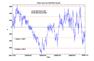
Many of us Canadians like to think of our economy as a member of the advanced, post-industrial world, with the landscape dotted with brand-name companies such as Nortel Networks, Research In Motion, and Four Seasons Hotels. In the back of our minds, of course, we know we are also a resource-rich country. But still, it may come as a bit of an embarrassment to find out that, of all the sector index funds we can compare the MSCI Canada Index fund EWC to, it cointegrates only with the natural resource index fund IGE. Even the financial sector indices do not come close, despite the presence of numerous financial services companies in the Canada Index. As usual, in the chart below, I plotted the spread between 100 shares of IGE and 400 shares of EWC, and we can see for ourselves how this spread stubbornly sticks close to zero.






One may note that IGE also cointegrates with the Emerging Markets index fund EEM. (The chart below is the spread between 100 shares of IGE and 100 shares of EEM.)


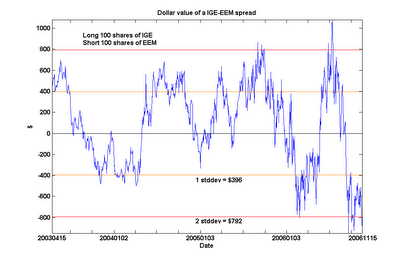This is not surprising. But does this imply the unsettling conclusion that the Canadian economy cointegrates with the emerging markets? No. I will not bore you with yet another chart: just be assured that cointegration is not a transitive relation.

Trading a platinum-gold seasonal spread

Quantitative traders can sometimes lose sight of the fact that many profitable trading strategies are extremely simple, requiring no math at all. Such is the case with a seasonal spread trade between platinum and gold that was profitable in all but one of the last 7 years. This is far more consistent than the seasonal spread trade that ruined Amaranth (see my earlier article).

The strategy is extremely simple: buy 2 July contracts of PL and short 1 June contract of GC around the end of February, and exit the positions around mid-April. (The gold futures contract specifies 100 ounces, while platinum is only 50, therefore we need to buy 2 contracts of PL vs. 1 contract of GC.) I first read about this strategy in an article by Jerry Toepke in the SFO Magazine in the beginning of 2006 and I decided not only to backtest it, but also paper trade this strategy in 2006 to see if it works its magic again. Both the backtest and the paper trade worked as advertised, despite being widely publicized by the magazine. I plot the P/L in this chart:


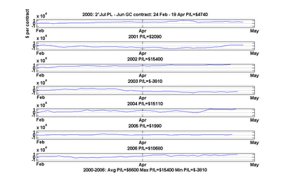
This spread earned an average of $6,600 every year since 1995. We earned $15,400 in the best year, while in the worst year we lose only $3,810. With a margin requirement of only $743 for trading this spread at NYMEX, the return per trade is not bad!

What is the fundamental reason this seasonal spread works? Amusingly, it has to do with the end of the Chinese New Year. According to Mr. Toepke, the demand for gold is driven by demand for jewelry. Asian countries such as India and China are the largest consumers of gold. A series of festivals and celebrations in these countries around year-end lasted till the end of the Chinese New Year in February, after which demand for delivery of gold is seasonally exhausted. Platinum, on the other hand, is primarily used in catalytic converters for automobiles, and the seasonality is much weaker. It is therefore handy as a hedge for gold prices.

Further reading: Jerry Toepke, “Give Seasonal Spreads Some Respect”, Stocks, Futures and Options Magazine, January 2006 issue.

Cointegration of OIH with spot oil price

Both my friend Yaser Anwar over at the Investment Ideas blog and my reader Jim urged me to test the oil services ETF OIH instead of XLE for cointegration with crude oil price. Their reasoning is that OIH is composed of oil drilling companies such as Schlumberger and Baker Huhges, as opposed to XLE, which is composed of oil-production companies like Exxon. The oil-drillers are more cyclical and react more to spot oil price rather than far futures contract prices. The hope is that OIH will tend to cointegrate better with spot oil price than XLE because of this. The fact that OIH has higher volatility as a result is not a concern to the arbitrageur (as opposed to the hedger), who profits from high volatility. In any case, its volatility should “cancel out” that of the spot oil price and result in a spread that may actually be less volatile. I follow their advice and carry out the analysis of CL vs. OIH.

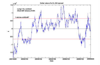
The plot is of the dollar value of long 1 contract of Cl and short 497 shares of OIH. They do cointegrate with over 90% probability. (I also plotted the 1 standard deviation lines of the spread to facilitate those who want to look for approximate entry points.) The cointegration probability is not measurably better than that between CL and XLE. However, the current spread (as of the close of Nov 20) is undervalued by only $9,617 (or 1.48 standard deviation), as opposed to $10,508 (or 1.74 standard deviation) for the CL-XLE spread. (I determined the standard deviation of the CL-XLE spread to be about $6,040). So in recent months, one can indeed say that OIH is trading more in line with spot oil price than XLE. But as an arbitrageur who thinks the larger the spread, the bigger the profit opportunity, this is not an endorsement for buying the CL-OIH spread instead. Rather, I would consider adding this spread as a means of diversification.

Thanks, Yaser and Jim, for this suggestion!

Extended analysis of energy futures and stocks arbitrage

A reader of my article “An arbitrage trade between energy stocks and futures” suggested that I should look at a longer history of crude oil prices vs. XLE. So I performed the same cointegration analysis for the front-month crude oil futures contract CL vs. XLE since December 1998. (I use CL instead of QM, the mini crude oil contract, due to its longer history.) Here is the plot of the dollar value of long 1 contract of CL and short 1,217 shares of XLE. (My previous analysis called for 1 contract of QM vs. 640 shares of XLE. The difference in shares is due to the half-size of QM relative to CL, and also to the larger dataset here.)

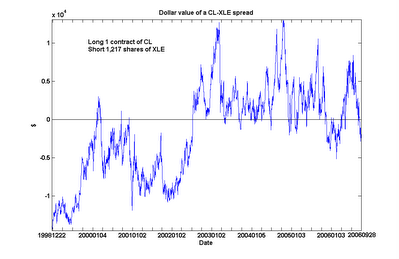An interesting feature emerged from this extended analysis. CL and XLE are still found to be cointegrated over this long period, albeit with a slightly lower probability (90%). However, we can see something of a regime shift around mid-2002, when CL went from generally under-valued to over-valued relative to XLE. (Even after including this regime with lower relative crude oil prices in my calculations, I still find the current spread to be undervalued by about $10,521 as of the close of Nov 17, which is near its 6-year low.)

What was the reason for this apparent shift in mid-2002? And are we in the middle of a similar regime shift in the opposite direction? Maybe our readers who have a better grasp of the economic fundamentals of the energy markets can shed light on this.

Email subscription to my blog now available

Instead of checking this blog constantly for new postings, you can now sign up to receive an email whenever a new article appears. Please see the "Enter your email" box on the right sidebar. You can of course unsubscribe at anytime, and your email will not be shared with anyone else without your permission.

Correction: Maximizing Compounded Rate of Return

A few readers pointed out a typo and an arithmetic error in my article "Maximizing Compounded Rate of Return". In the geometric random walk example where the stock can go up or down 1% at every step, the mean rate of return m is 0%, (not 1%), and the compounded rate of return is -0.005% (not -0.5%). My sincere thanks to all my readers who mercilessly scrutinize my ideas and check my numbers!

Reader suggested a possible trading strategy with the GLD - GDX spread

Steve Hansen of Raymond James Ltd. in Vancouver, B.C. suggested to me that a good trading signal for the GLD - GDX spread is when it exceeds 2 standard deviations from its mean. He observed that these are roughly at +/- $250 based on my definition of the spread, and that there were 3 such (immensely profitable) signals since the inception of GDX. Here is Mr. Hansen's plot:





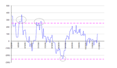
This certainly looks like a fairly safe strategy. Of course, if one desires more frequent signals, one can always enter into smaller positions at smaller spread values.

By the way, just when we were celebrating the reversion of the GLD - GDX spread this morning, the QM - XLE spread plunged to another multi-year low. With crude oil prices down about 30% from its all-time-high, XLE, the energy stocks ETF, is still within 5% of its all-time high. Does this make any sense? We shall see after this quarter's earnings from the oil companies are announced ...

GLD-GDX spread reverted to 0 this morning

Just a quick note on the GLD-GDX spread that I have been talking about. This morning (Nov 17) the negative spread completely reverted and has gone into positive territory.

An updated analysis of the arbitrage between gold and gold-miners

In my article about the arbitrage opportunity between gold and gold-miners, I cautioned that we should take the analysis with a grain of salt because of the short history of GDX (a gold-miners ETF). Adam Phillips of Van Eck Global, the firm which created GDX, has kindly pointed out to me that GDX is designed to track the Amex Gold Miners Index, GDM, which has a much longer history. Hence I repeated the analysis with gold spot prices vs. GDM for the last 3 years. The results confirm my earlier analysis with much higher statistical significance: GDM cointegrates with gold prices with over 99% probability. Here I plot the difference between the spot prices of 6.1 troy ounce of gold and the GDM index multiplied by 3.68 (to compare with my earlier plot, I normalize the gold prices and the GDM index so that the Gold-GDM spread yields roughly the same dollar value as the GLD-GDX spread at any time):

The mean-reversion of this spread is even more obvious than my plot in the earlier article. Also, with the longer history, we get a much better feel for the range of fluctuations. While the value of the spread is about -$213 as of the close of Nov 9, it can certainly go much lower before reverting, based on the highs and lows of the last 3 years.


FOOTNOTE

A reader of my earlier article made an interesting comment about shorting ETF’s such as GDX and GLD. He argued that since ETF shares can be constantly created, it should not require existing shares to be borrowed for shorting. I asked Mr. Phillips of Van Eck Global about this, and he confirmed to me that a newer ETF like GDX can in fact be hard to borrow. He went on to say that the borrowing of ETF’s has nothing to do with the issuer. The issuer can indeed create an unlimited supply of the shares, but the trader still need to borrow them from his or her broker for shorting. He also told me he is currently working hard to eliminate any borrowing problems in GDX that may have existed.