Conditional Portfolio Optimization: Using machine learning to adapt capital allocations to market regimes

By Ernest Chan, Ph.D., Haoyu Fan, Ph.D., Sudarshan Sawal, and Quentin Viville, Ph.D.

Previously on this blog, we wrote about a machine-learning-based parameter optimization technique we invented, called Conditional Parameter Optimization (CPO). It appeared to work well on optimizing the operating parameters of trading strategies, but increasingly, we found that its greatest power lies in its potential to optimize portfolio allocations. We call this Conditional Portfolio Optimization (which fortuitously shares the same acronym).

Let’s recap what Conditional Parameter Optimization is. Traditionally, optimizing the parameters of any business process (such as a trading strategy) is a matter of finding out what parameters give an optimal outcome over past data. For example, setting a stop loss of 1% gave the best Sharpe ratio for a trading strategy backtested over the last 10 years. Or running the conveyor belt at 1m per minute led to the lowest defect rate in a manufacturing process. Of course, the numerical optimization procedure can become quite complicated based on a number of different factors. For example, if the number of parameters is large, or if the objective function that relates the parameters to the outcome is nonlinear, or if there are numerous constraints on the parameters. There are already standard methods to handle these difficulties. 

What concerns us at PredictNow.ai, is when the objective function is not only nonlinear, but also depends on external time varying and stochastic conditions. In the case of a trading strategy, the optimal stop loss may depend on the market regime, which may not be clearly defined. In the case of a manufacturing process, the optimal conveyor belt rate may depend on dozens of sensor readings. Such objective functions mean that traditional optimization methods do not usually give the optimal results under a particular set of external conditions.Furthermore, even if you specify that exact set of conditions, the outcome is not deterministic. What better method than machine learning to solve this problem!

By using machine learning,  we can approximate this objective function using a neural network, by training its many nodes using historical data. (Recall that a neural network is able to approximate almost any function, but you can use many other machine learning algorithms instead of neural networks for this task). The inputs to this neural network will not only include the parameters that we originally set out to optimize, but also the vast set of features that measure the external conditions. For example, to represent a “market regime”, we may include market volatility, behaviors of different market sectors, macroeconomic conditions, and many other input features. To help our clients efficiently run their models, Predictnow.ai provides hundreds of such market features. The output of this neural network would be the outcome you want to optimize. For example, maximizing the future 1-month Sharpe ratio of a trading strategy is a typical outcome. In this case you would feed historical training samples to the neural network that include the trading parameters, the market features, plus the resulting forward 1-month Sharpe ratio of the trading strategy as “labels” (i.e. target variables). Once trained, this neural network can then predict the future 1-month Sharpe ratio based on any hypothetical set of trading parameters and the current market features. 

With this method, we “only need” to try different sets of hypothetical parameters to see which gives the best Sharpe ratio and adopt that set as the optimal. We put “only need” in quotes because of course if the number of parameters is large, it can take very long to try out different sets of parameters to find the optimal. Such is the case when the application is portfolio optimization, where the parameters represent the capital allocations to different components of a portfolio. These components could be stocks in a mutual fund, or trading strategies in a hedge fund. For a portfolio that holds S&P 500 stocks, for example, there will be up to 500 parameters. In this case, during the training process, we are supposed to feed into the neural network all possible combinations of these 500 parameters, plus the market features, and find out what the resulting 5- or 20-day return, or Sharpe ratio, or whatever performance metric we want to maximize. All possible combinations? If we represent the capital weight allocated to each stock as w ∈ [0, 1], assuming we are not allowing short positions, the search space has w500=[0, 1]500 combinations, even with discretization, and our computer will need to run till the end of the universe to finish. Overcoming this curse of dimensionality is one of the major breakthroughs the Predictnow.ai team has accomplished with Conditional Portfolio Optimization.

To measure the value Conditional Portfolio Optimization adds, we need to compare it with alternative portfolio optimization methods. The default method is Equal Weights: applying equal capital allocations to all portfolio components. Another simple method is the Risk Parity method, where the capital allocation to each component is inversely proportional to its returns’ volatility. It is called Risk Parity because each component is supposed to contribute an equal amount of volatility, or risk, to the overall portfolio’s risk. This assumes zero correlations among the components’ returns, which is of course unrealistic. Then there is the Markowitz method, also known as Mean-Variance optimization. This well-known method, which earned Harry Markowitz a Nobel prize, maximizes the Sharpe ratio of the portfolio based on the historical means and covariances of the component returns. The optimal portfolio that has the maximum historical Sharpe ratio is also called the tangency portfolio. I wrote about this method in a previous blog post. It certainly doesn’t take into account market regimes or any market features. It is also a vagrant violation of the familiar refrain, “Past Performance is Not Indicative of Future Results”, and is known to produce all manners of unfortunate instabilities (see here or here). Nevertheless, it is the standard portfolio optimization method that most asset managers use. Finally, there is the Minimum Variance portfolio, which uses Markowitz’s method not to maximize the Sharpe ratio, but to minimize the variance (and hence volatility) of the portfolio. Even though this does not maximize its past Sharpe ratio, it often results in portfolios that achieve better forward Sharpe ratios than the tangency portfolio! Another case of “Past Performance is Not Indicative of Future Results”.

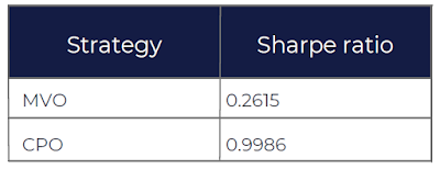
Let’s see how our Conditional Portfolio Optimization method stacks up against these conventional methods.  For an unconstrained optimization of the S&P 500 portfolio, allowing for short positions and aiming to maximize its 7-day forward Sharpe ratio, 

Method	Sharpe Ratio
Markowitz	0.31
CPO	0.96

(These results are over an out-of-sample period from July 2011 to June 2021, and the universe of stocks for the portfolio are those that have been present in the SP 500 index for at least 1 trailing month. The Sharpe Ratio we report in this and the following tables are all annualized). CPO improves the Sharpe ratio over the Markowitz method by a factor of 3.1.

Then we test our CPO performs for an ETF (TSX: MESH) given the constraints that we cannot short any stock, and the weight w of each stock obeys w ∈ [0.5%, 10%],

Period	Method	Sharpe Ratio	CAGR
2017-01 to 2021-07	Equal Weights	1.53	43.1%
	Risk Parity	1.52	39.9%
	Markowitz	1.64	47.2%
	Minimum Variance	1.56	38.3%
	CPO	1.62	43.6%
2021-08 to 2022-07	Equal Weights	-0.76	-30.6%
	Risk Parity	-0.64	-22.2%
	Markowitz	-0.94	-30.8%
	Minimum Variance	-0.47	-14.5%
	CPO	-0.33	-13.7%

CPO performed similarly to the Markowitz method in the bull market, but remarkably, it was able to switch to defensive positions and has beaten the Markowitz method in the bear market of 2022. It improves the Sharpe ratio over the Markowitz portfolio by more than 60% in that bear market. That is the whole rationale of Conditional Portfolio Optimization - it adapts to the expected future external conditions (market regimes), instead of blindly optimizing on what happened in the past. 

Next, we tested the CPO methodology on a private investor’s tech portfolio, consisting of 7 US and 2 Canadian stocks, mostly in the tech sector. The constraints are that we cannot short any stock, and the weight w of each stock obeys w ∈ [0%, 25%],

Period	Method	Sharpe Ratio	CAGR
2017-01 to 2021-07	Equal Weights	1.36	31.1%
	Risk Parity	1.33	24.2%
	Markowitz	1.06	23.3%
	Minimum Variance	1.10	19.3%
	CPO	1.63	27.1%
2021-08 to 2022-07	Equal Weights	0.39	6.36%
	Risk Parity	0.49	7.51%
	Markowitz	0.40	6.37%
	Minimum Variance	0.23	2.38%
	CPO	0.70	11.0%

CPO performed better than both alternative methods under all market conditions. In particular, it improves the Sharpe ratio over the Markowitz portfolio by 75% in the bear market.

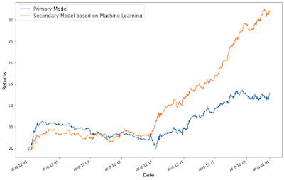
We also tested how CPO performs for some unconventional assets - a portfolio of 8 crypto currencies, again allowing for short positions and aiming to maximize its 7-day forward Sharpe ratio,

Method	Sharpe Ratio
Markowitz	0.26
CPO	1.00

(These results are over an out-of-sample period from January 2020 to June 2021, and the universe of cryptocurries for the portfolio are BTCUSDT, ETHUSDT, XRPUSDT, ADAUSDT, EOSUSDT, LTCUSDT, ETCUSDT, XLMUSDT). CPO improves the Sharpe ratio over the Markowitz method by a factor of 3.8.

Finally, to show that CPO doesn’t just work on portfolios of assets, we apply it to a portfolio of FX trading strategies traded live by a proprietary trading firm WSG. It is a portfolio of 7 trading strategies, and the allocation constraints are w ∈ [0%, 40%],

Method	Sharpe Ratio
Equal Weights	1.44
Markowitz	2.22
CPO	2.65

(These results are over an out-of-sample period from January 2020 to July 2022). CPO improves the Sharpe ratio over the Markowitz method by 19%.

In all 5 cases, CPO was able to outperform the naive Equal Weights portfolio and the Markowitz portfolio during a downturn in the market, while generating similar performance during the bull market.

For clients of our CPO technology, we can add specific constraints to the desired optimal portfolio, such as average ESG rating, maximum exposure to various sectors, or maximum turnover during portfolio rebalancing. The only input we require from them is the historical returns of the portfolio components (unless these components are publicly traded assets, in which case clients only need to tell us their tickers). Predictnow.ai will provide pre-engineered market features that capture market regime information. If the client has proprietary market features that may help predict the returns of their portfolio, they can merge those with ours as well. Clients’ features can remain anonymized. We will be providing an API for clients who wish to experiment with various constraints and their effects on the optimal portfolio.

If you’d like to learn more, please join us for our Conditional Portfolio Optimization webinar on Thursday, October 22, 2022, at 12:00 pm New York time. Please register here.

In the meantime, if you have any questions, please email us at info@predictnow.ai.

The demise of Zillow Offers: it is not AI's fault!

The story is now familiar: Zillow Group built a home price prediction system based on AI in order  to become a market-maker in the housing industry. As a market maker, the goal is simply to buy low and sell high, quickly, and with minimal transaction cost. Backtests showed that its AI model's predictive accuracy was over 96% (Hat tip: Peter U., for that article). In reality, though, it lost half a billion dollars.

This is a cautionary tale for anyone using AI to predict prices or returns, including those of us in more liquid markets than housing. Despite Zillow’s failure, the root cause of this discrepancy between backtest and live market-making is well-known, and it has nothing to do with machine learning or AI. Their failure was due to  adverse selection, which can happen to any market maker, whether human or machine. In this context, "market maker" is used in a broad sense - a market maker provides liquidity to the market using limit orders. For instance, any mean-reversion trader is a market maker. As long as the market maker is trading against a counterparty who has more information (a.k.a. the "informed trader"), adverse selection will take money away from the market maker and give it to the informed trader. This is because as market makers, the only model is to buy when prices are cheap, no matter why they are cheap. In contrast, the informed traders may know why the asset is cheap and if it will get cheaper, so they are happy to sell to a market maker. In the opposite situation, if the informed traders believe  that the current prices are cheap, but will get higher, they will refrain from selling. In this case, the limit order will not get executed, and market makers  suffer from "opportunity cost". In Zillow’s case, the informed traders are the homeowners who have a  better understanding of the value of their own home due to qualitative factors (e.g. views, interior design, neighborhood safety, etc.)  outside of Zillow’s model.

In my book Machine Trading, I wrote, "Adverse selection happens when prices on average go down after we buy something, and go up when we sell something". Therefore, adverse selection can be measured quite easily by computing the difference between the (paper) P&L of unfilled orders and the P&L of filled orders over a short time frame. In order to determine whether your AI predictive model will work in reality, it is ideal to deploy it live in a small capacity, and measure the differences over time. If there is significant adverse selection, the trader  can always choose not to participate in the market. For example, it is legendary that high frequency traders stopped providing liquidity to the market during extreme events such as flash crashes. Traders  don't want to be the suckers at the game. Unfortunately for Zillow, they weren’t aware of the well-practiced art of market making.

Another common way to reduce adverse selection is to keep a close tab on your inventory. If, in a short period of time, inventory suddenly changes significantly compared to average trends, it may indicate that there is new information arriving on the market that you are not aware of (e.g. mortgage rate going up by 1%). In this situation, it would be wise to cancel your limit orders until the coast clears. For a mathematical interpretation of this concept, view the formulation by Avellaneda and Sasha. Inventory management was a key  technique that Zillow did not adopt, which could have minimized their adverse selection risk.

AI has been a major asset in numerous business processes, including market making, but it is just one part of complex production machinery. As we can see from Zillow’s use case, predictions, even accurate ones, are not enough to generate profits. As I explained in my previous blog post, we at Predictnow.ai don't think that AI is the be-all and end-all of decision making. Instead, we believe the value of AI lies in its ability to correct human-made decisions. But, an even larger lesson here is that experts in one industry (e.g. housing) can benefit from the knowledge of experts in another industry (e.g. quantitative finance). This transdisciplinary knowledge is exactly what Predictnow.ai offers enterprises to improve and enhance their processes.

800+ New Crypto Features

 By Quentin Viville, Sudarshan Sawal, and Ernest Chan

PredictNow.ai is excited to announce that we’re expanding our feature zoo to cover crypto features! This follows our work on US stock features, and features based on options activities, ETFs, futures, and macroeconomic indicators. To read more on our previous work, click here. These new crypto features can be used as input to our machine-learning API to help improve your trading strategy. In this blog we have outlined the new crypto features as well as demonstrated  how we have used them for short term alpha generation and crypto portfolio optimization.

Our new crypto features are designed to capture market activity  from subtle movements to large overarching trends. These features will quantify the variations of the price, the return, the order flow, the volatility and the correlations that appear among them.

To create these features, we first constructed the Base Features  using raw market data that includes microstructure information. Next, we applied simple mathematical functions such as exponential moving average to create the Final Features.

Base Features

The Base Features are constructed using Binance’s dollar bar data, which includes:

• Open
• High
• Low
• Close
• Volume
• Order flow (sum of signed volumes) 
• +ve volume for buy aggressor tag and -ve volume for sell aggressor tag
• Buy market order value (sum of volumes corresponding to buy aggressor tag)
• Sell market order value (sum of volumes corresponding to sell aggressor tag)

Base Features are based on:

1. Relations between the price, the high price, the low price.
• Relative High: High Price relative to Open Price.
• Relative Low: Low Price relative to Open Price.
• Relative Close: Close Price relative to Open Price.
• Relative Volume: Buy orders relative to total absolute volume.
• Target Effort: computes an estimation of the “effort” that the price has to produce to reach the target price by comparing the observed low price and high price.
2. Volume exchanged.
• Dollar Speed: Average signed quantity of dollars exchanged per second.
3. Relations and potential correlations among the variations of the price, the order flow and the intensity of the activity in the market.
• Kyle’s Lambda: Relation between price change and orderflow.
• SCOF: Correlation of Order Flow with its lagged series.
• VPIN: Volume-synchronized probability of informed trading. 
4. Volatility observed.
• VLT: Volatility of the returns (Exponentially Weighted)

Each feature is associated with a ‘time span’, or lookback period, which helps capture market activity across  multiple time frames.

Final Features

Once we generated the Base Features, a new, varied set of features was derived called the Final Features.These Final Features are transformations of the initial Base Features into exponentially moving averages and probabilities over many time periods.

This approach has allowed us to produce a large set of Final Features (879 features to be exact), which can capture and quantify the activity of the market within any time span we choose.

Applications to Short Term Alpha Generation

PredictNow.ai’s core functionality is metalabelling, which assigns a Probability of Profit for every trade of an existing strategy (or a future time period of an existing portfolio). This requires us to build a machine learning model using a large number of input features and a target (label), which would be the trades’ (or portfolio’s) returns.

To evaluate the performance of the features described above, we first built a base strategy and then applied metalabelling to the signals of that strategy with those features as input. The base strategy is a high frequency strategy which predicts abnormal returns due to unusual order flow. The out-of-sample backtest performance of just the base strategy:

Maximum drawdown: −6.250%

Annualized Sharpe ratio:3.3

Annualized profit: 32.6% 

Using the Final Features as described above as input to metalabelling, we have been successful in improving  the strategy’s performance drastically. The improved performance after applying metalabelling:

Maximum drawdown: −4.998%

Annualized Sharpe ratio: 5.6

Annualized profit: 227% 

Comparative plot to give an idea of the metalabelling model’s performance in comparison to the base strategy:

The Sharpe ratio is increased from 3.1 to 5.6 and we have almost 7x the annual returns to 227% by applying metalabelling using our new crypto features.

Applying CPO to Crypto Portfolio

Mean Variance Optimization (MVO) is a popular method of portfolio optimization which generates a portfolio with maximum expected returns given a fixed level of risk. One shortcoming of the MVO method is that the selected portfolio is optimal only on average in the past. This doesn’t guarantee it to be optimal in different market regimes. This limitation gives us an opportunity to apply our patent-pending Conditional Parameter Optimization (CPO) technique.

Our CPO technique can be used to improve strategy performance in different market regimes by adapting a trading strategy’s parameters to fit those regimes. Similarly, it can optimize allocations to different constituents of a portfolio in different market regimes. Rather than optimizing based only on the historical means and covariances of a portfolio’s constituents’ returns, CPO involves training a machine learning model with a vast number of external “big data” features to drive the optimization process.

In our next example, we used our crypto features as input. We then compared the Sharpe ratios of a crypto portfolio based on the conventional MVO technique vs our CPO technique on out-of-sample data.

Backtest Result:

• Portfolios are constituted of 8 symbols (all crypto perpetual futures): BTCUSDT, ETHUSDT, XRPUSDT, ADAUSDT, EOSUSDT, LTCUSDT, ETCUSDT, XLMUSDT
• Position type includes Long and Short Positions
• The target variable is the forward Sharpe ratio, computed as the 3-hour return divided by the standard deviation of the sequence of the 5-minute consecutive returns during the 3-hour period
• Out-of-sample test data set starts on Jan. 2020 and ends on June 2021
• Results (annualized Sharpe ratio over 365 days per year):

• CPO improves the Sharpe ratio by x3.8!

Conclusion

We have demonstrated that our new crypto features are powerful additions to any crypto trader or investor’s toolkit by applying them to a crypto trading strategy in live deployment, and to optimizing a crypto portfolio using our proprietary CPO technique. Our features and strategy combined with our machine learning software is proven to increase a base trading strategy’s returns by 7x and increase a crypto portfolio’s Sharpe ratio 3.8x over MVO. Additionally, with our Explainable AI function using our feature selection methodology, we’ve removed the guesswork so you’ll know exactly which of our new crypto features are important to improving your strategy.

To sign up for a free trial to experiment with these new features using our API or to explore our machine learning software please click here. Institutional investors can also inquire about subscribing to our trading signals from our crypto strategy or to updates from our dynamically optimized long-short crypto portfolio.

If you have any questions or would like to work with us, please email us at: info@predictnow.ai.