Quantitative traders can sometimes lose sight of the fact that many profitable trading strategies are extremely simple, requiring no math at all. Such is the case with a seasonal spread trade between platinum and gold that was profitable in all but one of the last 7 years. This is far more consistent than the seasonal spread trade that ruined Amaranth (see my earlier
article).
The strategy is extremely simple: buy 2 July contracts of PL and short 1 June contract of GC around the end of February, and exit the positions around mid-April. (The gold futures contract specifies 100 ounces, while platinum is only 50, therefore we need to buy 2 contracts of PL vs. 1 contract of GC.) I first read about this strategy in an article by Jerry Toepke in the SFO Magazine in the beginning of 2006 and I decided not only to backtest it, but also paper trade this strategy in 2006 to see if it works its magic again. Both the backtest and the paper trade worked as advertised, despite being widely publicized by the magazine. I plot the P/L in this chart:

This spread earned an average of $6,600 every year since 1995. We earned $15,400 in the best year, while in the worst year we lose only $3,810. With a margin requirement of only $743 for trading this spread at NYMEX, the return per trade is not bad!
What is the fundamental reason this seasonal spread works? Amusingly, it has to do with the end of the Chinese New Year. According to Mr. Toepke, the demand for gold is driven by demand for jewelry. Asian countries such as India and China are the largest consumers of gold. A series of festivals and celebrations in these countries around year-end lasted till the end of the Chinese New Year in February, after which demand for delivery of gold is seasonally exhausted. Platinum, on the other hand, is primarily used in catalytic converters for automobiles, and the seasonality is much weaker. It is therefore handy as a hedge for gold prices.
Further reading: Jerry Toepke, “Give Seasonal Spreads Some Respect”, Stocks, Futures and Options Magazine, January 2006 issue.
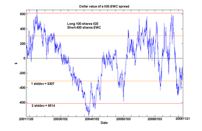
 This is not surprising. But does this imply the unsettling conclusion that the Canadian economy cointegrates with the emerging markets? No. I will not bore you with yet another chart: just be assured that cointegration is not a transitive relation.
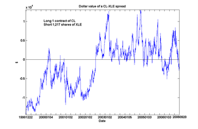 An interesting feature emerged from this extended analysis. CL and XLE are still found to be cointegrated over this long period, albeit with a slightly lower probability (90%). However, we can see something of a regime shift around mid-2002, when CL went from generally under-valued to over-valued relative to XLE. (Even after including this regime with lower relative crude oil prices in my calculations, I still find the current spread to be undervalued by about $10,521 as of the close of Nov 17, which is near its 6-year low.)


 Now consider stock A and stock C.
 Stock C clearly doesn’t move in any correlated fashion with stock A: some days they move in same direction, other days opposite. Most days stock C doesn’t move at all! But notice that the spread in stock prices between C and A always return to about $1 after a while. This is a manifestation of cointegration between A and C. In this instance, a profitable trade would be to buy A and short C at around day 10, then exit both positions at around day 19. Another profitable trade would be to buy C and short A at around day 31, then closing out the positions around day 40.