Simulating returns using either the traditional closed-form equations or probabilistic models like Monte Carlo has been the standard practice to match them against empirical observations from stock, bond and other financial time-series data. (See Chan and Ng, 2017 and Lopez de Prado, 2018.) Some of the stylised facts of return distributions are as follows:
- The tails of an empirical return distribution are always thick, indicating lucky gains and enormous losses are more probable than a Gaussian distribution would suggest.
- Empirical distributions of assets show sharp peaks which traditional models are often not able to gauge.
To generate simulated return distributions that are faithful to their empirical counterpart, I tried my hand on various kinds of Generative Adversarial Networks, a very specialised Neural Network to learn the features of a stationary series we’ll describe later. The GAN architectures used here are a direct descendant of the simple GAN invented by Goodfellow in his 2014 paper. The ones tried for this exercise were the conditional recurrent GAN and the simple GAN using fully connected layers. The idea involved in the architecture is that there are two constituent neural networks. One is called the Generator which takes a vector of random noise as input and then generates a time series window of a couple of days as output. The other component called Discriminator tries to take either this generated window as input or takes a real window of price returns or other features as input and tries to decipher whether a given window of returns or other features is “real” ( from the AAPL data) or “fake” (generated by the Generator). The job of the generator is to try to “fool” the discriminator by successively (as it is being trained) generating more “real” data. The training goes on until:
1) the generator is able to output the feature set which is identical in distribution to the real dataset on which both the networks were trained
2) The discriminator is able to tell real data from the generated one
The mathematical objectives of this training are to maximise:
a ) log(D(x)) + log(1 - D(G(z))) - Done by the discriminator - Increase the expected ( over many iterations ) log probability of the Discriminator D to identify between the real and fake samples x. Simultaneously, increase the expected log probability of discriminator D to correctly identify all samples generated by generator G using noise z.
b) log(D(G(z))) - Done by the generator - So, as observed empirically while training GANs, at the beginning of training G is an extremely poor “truth” generator while D quickly becomes good at identifying real data. Hence, the component log(1 - D(G(z))) saturates or remains low. It is the job of G to maximize log(1 - D(G(z))). What that means is G is doing a good job of creating real data that D isn’t able to “call out”. But because log(1 - D(G(z))) saturates, we train G to maximize log(D(G(z))) rather than minimize log(1 - D(G(z))).
Together the min-max game that the two networks play between them is formally described as:
minGmaxDV (D, G) =Epdata(x)[log D(x)] +E p(z) [log(1 − D(G(z)))]
The real data sample x is sampled from the distribution of empirical returns pdata(x)and the zis random noise variable sampled from a multivariate gaussian p(z). The expectations are calculated over both these distributions. This happens over multiple iterations.
The hypothesis was that the various GANs tried will be able to generate a distribution of returns which are closer to the empirical distributions of returns than ubiquitous baselines like Monte Carlo method using the Geometric Brownian motion.
The experiments
A bird’s-eye view of what we’re trying to do here is that we’re trying to learn a joint probability distribution across time windows of all features along with the percentage change in adjusted close. This is so that they can be simulated organically with all the nuances they naturally come together with. For all the GAN training processes, Bayesian optimisation was used for hyperparameter tuning.
In this exercise, initially, we first collected some features belong to the categories of trend, momentum, volatility etc like RSI, MACD, Parabolic SAR, Bollinger bands etc to create a feature set on the adjusted close of AAPL data which spanned from the 1980s to today. The window size of the sequential training sample was set based on hyperparameter tuning. Apart from these indicators the percentage change in the adjusted OLHCV data were taken and concatenated to the list of features. Both the generator and discriminator were recurrent neural networks ( to sequentially take in the multivariate window as input) powered by LSTMs which further passed the output to dense layers. I have tried learning the joint distributions of 14 and also 8 features The results were suboptimal, probably because of the architecture being used and also because of how notoriously tough the GAN architecture might become to train. The suboptimality was in terms of the generators’ error not reducing at all ( log(1 - D(G(z))) saturating very early in the training ) after initially going up and the random return distributions without any particular form being generated by the generators.
After trying conditional recurrent GANs, which didn’t train well, I tried using simpler multilayer perceptrons for both Generator and Discriminators in which I passed the entire window of returns of the adjusted close price of AAPL. The optimal window size was derived from hyperparameter tuning using Bayesian optimisation. The distribution generated by the feed-forward GAN is shown in figure 1.
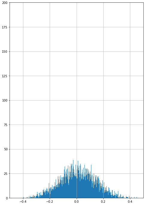
Fig 1. Returns by simple feed-forward GAN
Some of the common problems I faced were either partial or complete mode collapse - where the distribution either did not have a similar sharp peak as the empirical distribution ( partial ) or any noise sample input into the generator produces a limited set of output samples ( complete).
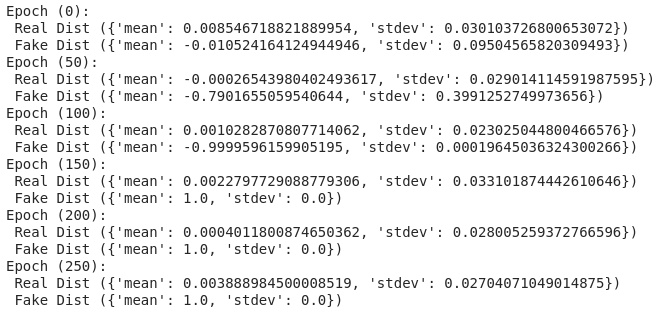
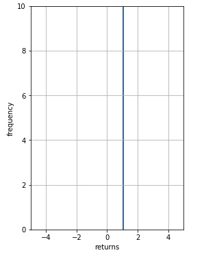
The figure above shows mode collapsing during training. Every subsequent epoch of the training is printed with the mean and standard deviation of both the empirical subset (“real data”) that is put into the discriminator for training and the subset generated by the generator ( “fake data”). As we can see at the 150th epoch, the distribution of the generated “fake data” absolutely collapses. The mean becomes 1.0 and the stdev becomes 0. What this means is that all the noise samples put into the generator are producing the same output! This phenomenon is called Mode Collapse as the frequencies of other local modes are not inline with the real distribution. As you can see in the figure below, this is the final distribution generated in the training iterations shown above:
A few tweaks which reduced errors for both Generator and Discriminator were 1) using a different learning rate for both the neural networks. Informally, the discriminator learning rate should be one order higher than the one for the generator. 2) Instead of using fixed labels like 1 or a 0 (where 1 means “real data” and 0 means “fake data”) for training the discriminator it helps to subtract a small noise from the label 1 and add a similar small noise to label 0. This has the effect of changing from classification to a regression model, using mean square error loss instead of binary cross-entropy as the objective function. Nonetheless, these tweaks have not eliminated completely the suboptimality and mode collapse problems associated with recurrent networks.
Baseline Comparisons
We compared this generated distribution against the distribution of empirical returns and the distribution generated via the Geometric Brownian Motion - Monte Carlo simulations done on AAPL via python. The metrics used to compare the empirical returns from GBM-MC and GAN were Kullback-Leibler divergence to compare the “distance” between return distributions and VAR measures to understand the risk being inferred for each kind of simulation. The chains generated by the GBM-MC can be seen in fig. 4. Ten paths were simulated in 1000 days in the future based on the inputs of the variance and mean of the AAPL stock data from the 1980s to 2019. The input for the initial price in GBM was the AAPL price on day one.
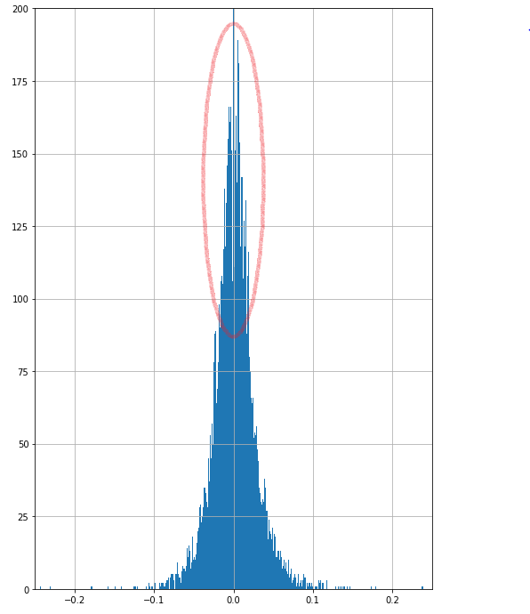
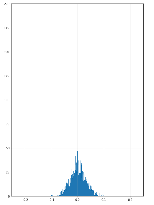
Fig 2. shows the empirical distributions for AAPL starting 1980s up till now. Fig 3. shows the generated returns by Geometric Brownian motion on AAPL.
To compare the various distributions generated in the exercise I binned the return values into 10,000 bins and then calculated the Divergence using the non-normalised frequency value of each bin. The code is:
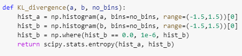
The formula scipy uses behind the scene for entropy is:
S = sum(pk * log(pk / qk)) where pk,qk are bin frequencies
The Geometric Brownian Motion generation is a better match for the empirical data compared to the one generated using Multiperceptron GANs even though it should be noted that both are extremely bad.
The VAR values ( calculated over 8 samples ) here tell us that beyond a confidence level, the kind of returns (or losses) we might get - in this case, it is the percentage losses with 5% and 1% chance given the distributions of returns:
The GBM generator VARs seem to be much closer to the VARs of the Empirical distribution.
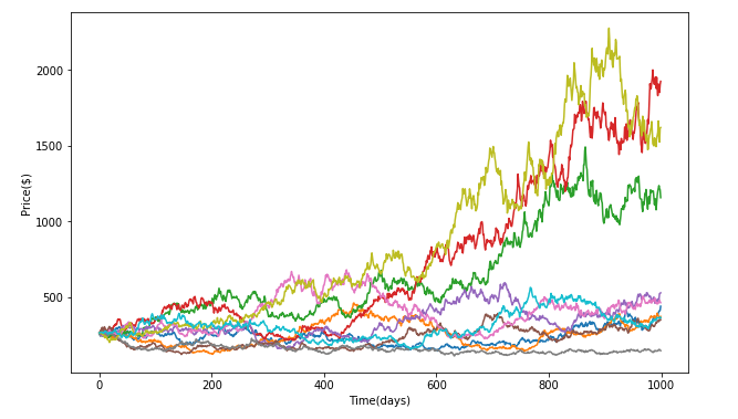
. Fig 4. Showing the various paths generated by the Geometric Brownian motion model using monte Carlo.
Conclusion
The distributions generated by both methods didn’t generate the sharp peak shown in the empirical distribution (figure 2). The spread of the return distribution by the GBM with Monte Carlo was much closer to reality as shown by the VAR values and its distance to the empirical distribution was much closer to the empirical distribution as shown by the Kulback-Leibler divergence, compared to the ones generated by the various GANs I tried. This exercise reinforced that GANs even though enticing are tough to train. While at it I discovered and read about a few tweaks that might be helpful in GAN training. Some of the common problems I faced were 1) mode collapse discussed above 2) Another one was the saturation of the generator and “overpowering” by the discriminator. This saturation causes suboptimal learning of distribution probabilities by the GAN. Although not really successful, this exercise creates scope for exploring the various newer GAN architectures, in addition to the conditional recurrent and multilayer perceptron ones which I tried, and use their fabled ability to learn the subtlest of distributions and apply them for financial time-series modelling. Our codes can be found at Github here. Any modifications to the codes that can help improve performance are most welcome!
About Author:
Akshay Nautiyal is a Quantitative Analyst at Quantinsti, working at the confluence of Machine Learning and Finance. QuantInsti is a premium institute in Algorithmic & Quantitative Trading with instructor-led and self-study learning programs. For example, there is an interactive course on using Machine Learning in Finance Markets that provides hands-on training in complex concepts like LSTM, RNN, cross validation and hyper parameter tuning.
Industry update
1) Cris Doloc published a new book “Computational Intelligence in Data-Driven Trading” that has extensive discussions on applying reinforcement learning to trading.
2) Nicolas Ferguson has translated the Kalman Filter codes in my book Algorithmic Trading to KDB+/Q. It is available on Github. He is available for programming/consulting work.
3) Brain Stanley at QuantRocket.com wrote a blog post on "Is Pairs Trading Still Viable?"
4) Ramon Martin started a new blog with a piece on "DeepTrading with Tensorflow IV".
5) Joe Marwood added my book to his top 100 trading books list.
6) Agustin Lebron's new book The Laws of Trading contains a good interview question on adverse selection (via Bayesian reasoning).
7) Linda Raschke's new autobiography Trading Sardines is hilarious!
5 comments:
Did you ever consider bootstrap? For timeseries and other dependent bootstrap you could use block bootstrap, stationary bootstrap and model-based bootstrap. Unlike Monte Carlo, fat tails can easily be simulated. And the statistical properties are well understood unlike GANs.
Dear Ernie,
Long time reader here. I recently chanced upon this article re: TS Stationarity and Memory.
https://towardsdatascience.com/non-stationarity-and-memory-in-financial-markets-fcef1fe76053
The mean reversion sections in your book Algorithmic Trading was the first thing that came to my mind. I don't necessarily have an opinion formed as of now.
Just curious about what you reckon?
Regards,
M
Thanks for the reference, M! I will take a look.
Ernie
M,
Yves-Laurent Kom Samo wrote in that article that no matter how long, one cannot test whether a time series is nonstationary. However, the example he gave is that a short section of a time series is nonstationary, but a longer section will show that it is stationary after all. That doesn't seem to support his claim?
Ernie
Ernie,
Thank you for your reply, Ernie. I agree that is what Samo showed in the first section. I gathered that the case he was trying to build was that memory and stationarity are separate testable qualities of a TS.
Which is goes against a lot of what Prado wrote about in his book Advances in Financial Machine Learning. Where he achieved TS stationarity using a binomial series of alternating weight signs to difference each obs(modified from the ARFIMA process, Hosking 1981 If I recall correctly).
It set off some alarms in me as it seemed too elegant and good to be true hence I sought your opinion.
Nonetheless, thank you for your reply once again and I eagerly look forward to your next book and the heuristics to be gleaned.
Warm Regards,
M
Post a Comment